
A worklog from optimizing an NVFP4 grouped GEMM kernel for GPUMode's Blackwell competition.
GPUMode recently ran a Blackwell kernel competition covering several NVFP4 GEMM-like workloads. I submitted to both the Dual GEMM and Grouped GEMM tracks.
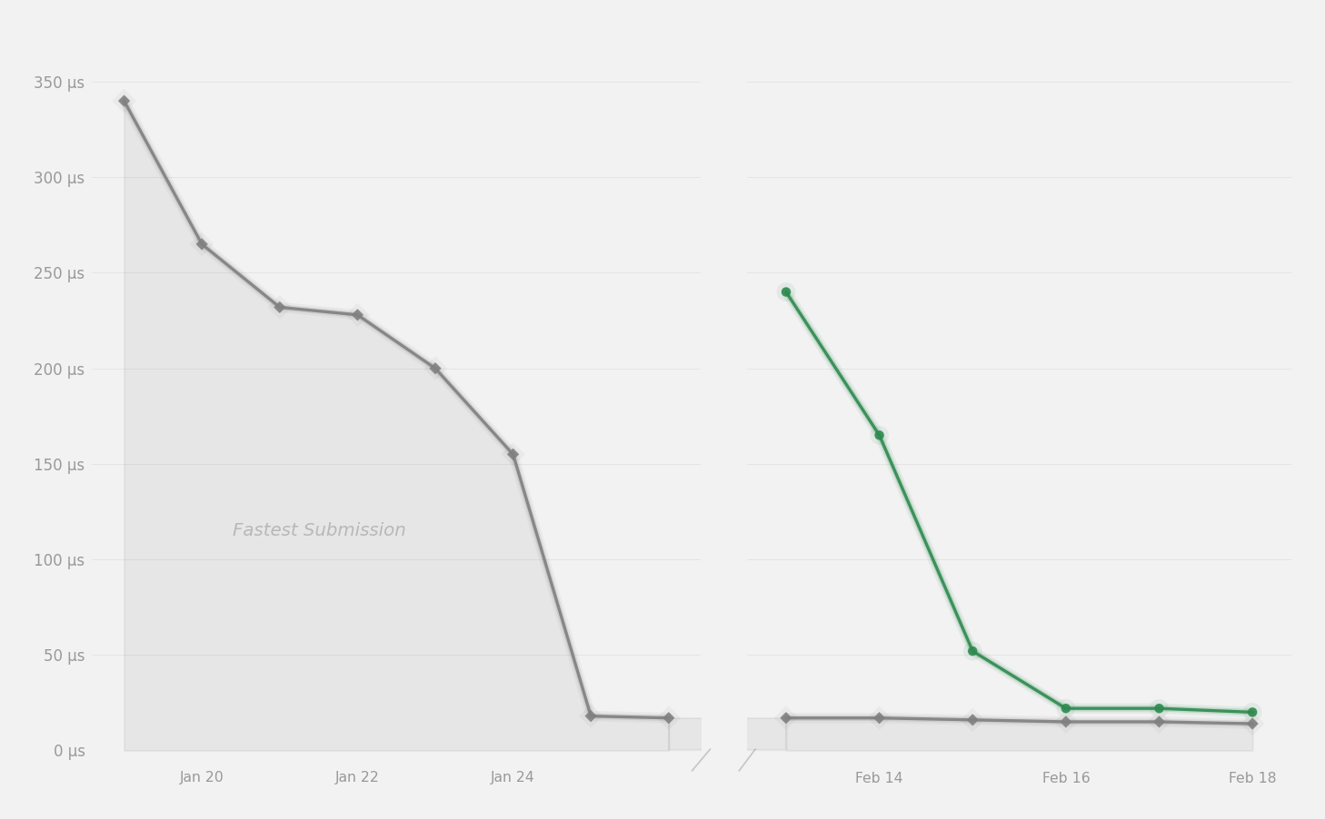
On the Grouped GEMM problem, my final kernel placed 6th on the NVIDIA leaderboard and 18th on the Modal leaderboard. The reference implementation had a 238 µs geometric mean; my final submission reached 23.8 µs. Most of the improvement came from removing host-side serialization, then tightening the device pipeline with TMA, warp specialization, thread block clusters, and multicast.
Background
The kernel is easier to follow with two pieces of context: grouped GEMM and NVFP4.
Grouped GEMM and MoE
In Mixture-of-Experts transformers, a gating network routes each token to one or more experts. The routing distribution changes from batch to batch, so each expert receives a different number of tokens.
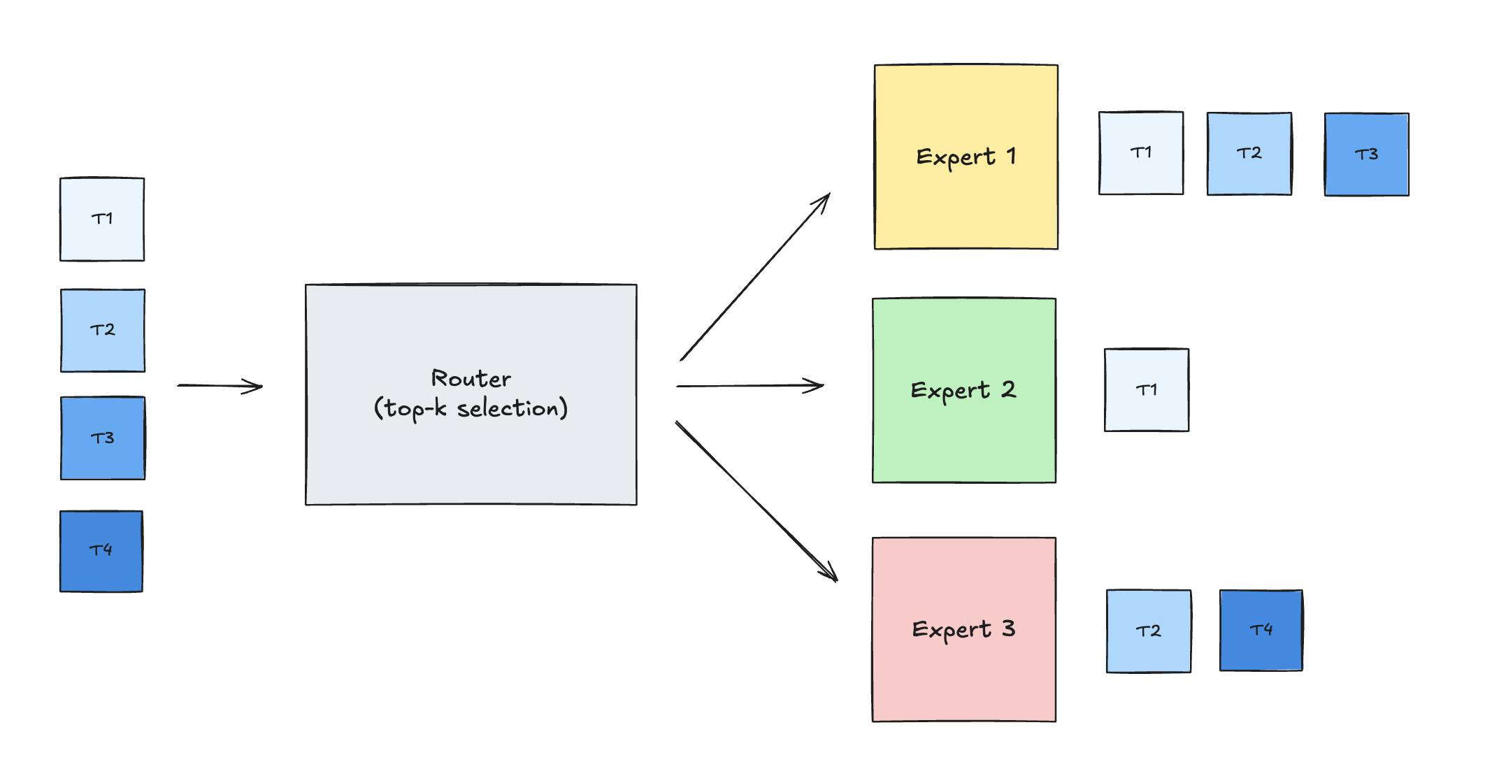
After top-k routing, tokens are reorganized by expert, creating variable-sized per-expert input batches.
The sequence dimension M is expert-specific: it is the number of tokens routed to a given expert. The projection dimensions K (input hidden size) and N (expert intermediate size) stay fixed across the layer.
The MoE forward pass decomposes into independent GEMM operations, one per expert, all sharing K and N but with different M values.
Referring to the routing diagram above:
| Expert | Tokens | GEMM |
|---|---|---|
| 1 | T1, T2, T3 | M=3 |
| 2 | T1 | M=1 |
| 3 | T2, T4 | M=2 |
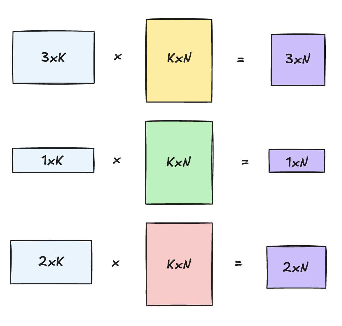
Each expert receives a different number of tokens, so the GEMMs have different M dimensions, while K and N are shared across experts for a given projection.
A grouped GEMM is one GPU kernel launch that executes a list of independent GEMMs. In MoE, each dispatched expert gets its own token subset, so each expert becomes one entry in the launch list.
For expert e, the FFN projection is:
1Y_e = X_e @ W_e
where X_e contains activations for tokens routed to expert e, W_e is the expert's weight matrix, and Y_e is the output. A grouped GEMM bundles these into one batched computation:
1{ X_1 @ W_1, X_2 @ W_2, X_3 @ W_3, ... }
Instead of paying launch overhead for each expert, grouped GEMM combines the problems into one launch. The host passes an array of descriptors:
1(A_1, B_1, C_1, M_1, N, K)
2(A_2, B_2, C_2, M_2, N, K)
3(A_3, B_3, C_3, M_3, N, K)
At the kernel level, each expert's output matrix is partitioned into block-level tiles. Those tiles are merged into one flattened work queue, so SMs can interleave work from different experts instead of draining one irregular problem at a time.
NVFP4
Blackwell introduced NVFP4 for low-precision inference. Quantizing weights and activations to 4 bits reduces memory traffic and increases effective tensor-core throughput, while block-level scaling recovers enough dynamic range for inference.
At the bit level, NVFP4 is an E2M1 representation (1 sign bit, 2 exponent bits, and 1 mantissa bit), yielding an effective dynamic range of approximately -6 to 6.
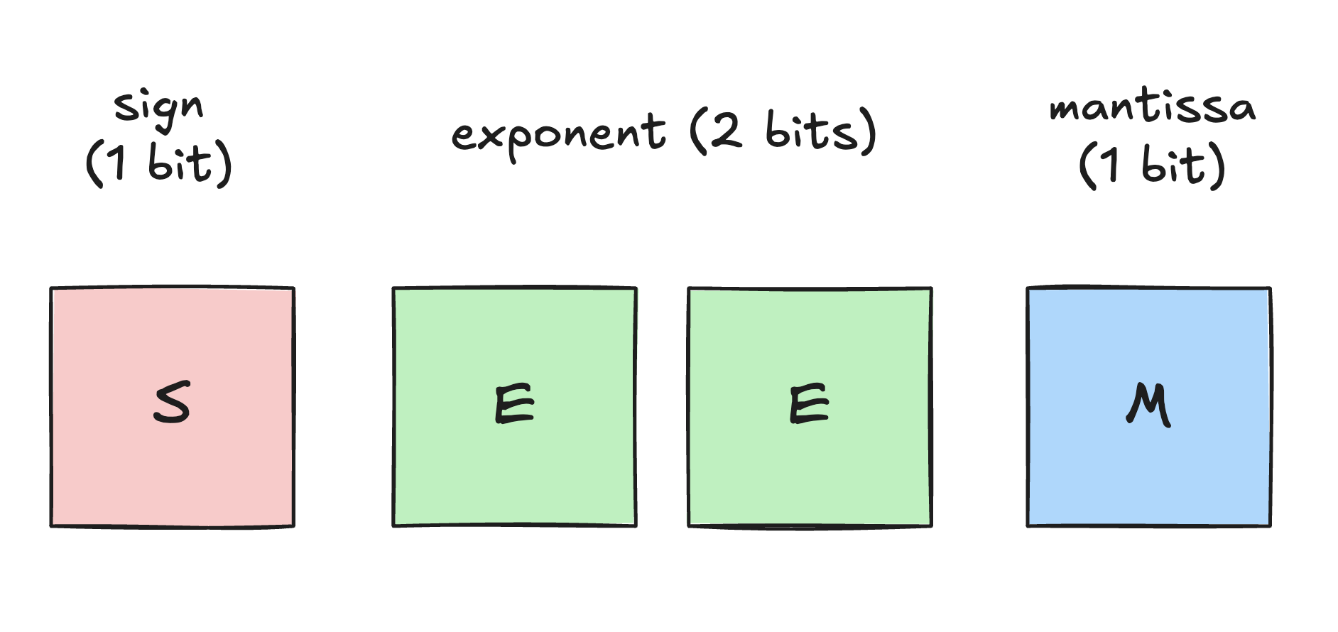
Four bits do not provide much dynamic range on their own, so NVFP4 relies on block-level scaling. Every block of 16 elements gets a higher-precision scale factor. Dequantization is effectively x_fp = x_nvfp4 * scale.
For the kernel, each operand has two memory streams: the quantized matrix (A or B) and its scale factors (SFA or SFB). Both must reach shared memory before the MMA can issue.
Kernel Worklog
The competition evaluated kernels on four input shapes, and I use these same shapes throughout the post.
Shape A - Deep-K
1g=8, K=7168, N=4096, mixed M=[80,176,128,72,64,248,96,160]
Large K and small M make each tile spend most of its time in the K-loop. Shape A mainly tests whether the producer/consumer pipeline can stay overlapped for many iterations.
Shape B - Wide-N
1g=8, K=2048, N=7168, mixed M=[40,76,168,72,164,148,196,160]
Large N and small M make memory bandwidth dominated by streaming matrix B and its scale factors. Shape B stresses wide-N behavior, B/SFB traffic, and work distribution across many tiles.
Shape C - Mid-sized
1g=2, K=4096, N=3072, M=[192,320]
Here M, N, and K are all moderately large. It is a useful sanity check: mainloop improvements should show up in end-to-end latency, not only in the pathological shapes.
Shape D - Shorter-K
1g=2, K=1536, N=4096, M=[128,384]
The short inner loop makes fixed costs dominate: CPU launch overhead, pipeline drain, and the final memory-write phase (the epilogue).
The final kernel is about 10x faster by geometric mean. All timings below are in microseconds.
| Version | Shape A | Shape B | Shape C | Shape D | Geo mean |
|---|---|---|---|---|---|
v1 | 641 | 451 | 142 | 80.2 | 240 |
v2 | 313 | 286 | 111 | 63.7 | 159 (-34%) |
v3 | 129 | 128 | 43.6 | 22.6 | 63.5 (-60%) |
v4 | 47.5 | 45.0 | 14.3 | 10.5 | 23.8 (-63%) |
Kernel reference
The competition organizers provided a CuTeDSL reference:
| Version | Shape A | Shape B | Shape C | Shape D |
|---|---|---|---|---|
| Reference | 351 µs | 341 µs | 167 µs | 146 µs |
The geometric mean is 238 µs. That is the baseline for the rest of the post.
v1: Correctness-First Baseline
My first version (v1) was a correctness-first CUDA/C++ port of the reference kernel. It used TMA (Tensor Memory Accelerator) to asynchronously bulk-load tiles from global memory into shared memory.
To hide memory latency, I set up a 2-stage software pipeline using asynchronous mbarriers to overlap TMA loads with tensor-core compute.
For compute, I used tcgen05.mma for mixed-precision NVFP4 math. It writes accumulators directly into Tensor Memory (TMEM), avoiding accumulator pressure on regular registers.
Host-side
To use Blackwell's Tensor Memory Accelerator, the kernel must describe the operand layout to the hardware. TMA does this through Tensor Map descriptors rather than raw pointers.
1// Host-side Tensor Map descriptor for a tiled NVFP4 operand.
2cuTensorMapEncodeTiled(
3    &tmap,
4    CUtensorMapDataType::CU_TENSOR_MAP_DATA_TYPE_16U4_ALIGN8B,
5    3, (void*)ptr, globalDim, globalStrides, boxDim, elementStrides,
6    /* config flags */
7);
For this kernel, the descriptor fields that matter are the global tensor shape, global strides, and tile shape. Encoding them on the CPU moves index arithmetic and out-of-bounds handling into dedicated hardware on the GPU.
Bulk Asynchronous Data Loads
On the device side, a single thread issues a hardware command to move an entire 2D or 3D tile with TMA. The usual alternative is a cooperative load where each thread moves a few bytes into SMEM.
1__device__ inline void tma_3d_gmem2smem(
2    int dst_smem, const void *tmap_ptr, int x, int y, int z, int mbar_addr) {
3  asm volatile(
4    "cp.async.bulk.tensor.3d.shared::cta.global.mbarrier::complete_tx::bytes... "
5    "[%0], [%1, {%2, %3, %4}], [%5], %6;"
6    :: "r"(dst_smem), "l"(tmap_ptr), "r"(x), "r"(y), "r"(z), "r"(mbar_addr) ...
7  );
8}
The cp.async.bulk.tensor PTX instruction tells the TMA engine to fetch a sub-tile directly from global memory to shared memory (dst_smem). The transfer runs asynchronously and signals a hardware barrier (mbarrier_addr) on completion.
Computing the MMA
Once the FP4 data and scale factors are in shared memory, the kernel passes them to the tensor cores (tcgen05).
1__device__ __forceinline__ void tcgen05_mma_nvfp4(
2  int d_tmem, uint64_t a_desc, uint64_t b_desc, ...
3) {
4  asm volatile(
5    "tcgen05.mma.cta_group::1.kind::mxf4nvf4.block_scale.block16 "
6    "  [%0], %1, %2, %3, [%4], [%5], p;"
7    :: "r"(d_tmem), "l"(a_desc), "l"(b_desc) ...
8  );
9}
The destination accumulator ([%0] / d_tmem) is not a standard GPU register. It points to TMEM (Tensor Memory), a specialized on-chip memory space for accumulated matrix results.
Double-buffered main loop
The baseline overlaps memory fetches (TMA) and math (MMA) with a two-stage software pipeline.
1for (int k_iter = 0; k_iter < num_k_iters; k_iter++) {
2  int stage = k_iter % 2;
3  int next_stage = (k_iter + 1) % 2;
4
5  // Wait for the hardware barrier to confirm TMA has loaded 'stage'
6  if (tid == 0) mbarrier_wait(tma_mbar[stage], phase);
7  __syncthreads();
8
9  // Tell TMA to start fetching the *next* block of data in the background
10  if (tid == 0) issue_tma_loads(..., next_stage);
11
12  // Command tensor cores to multiply the *current* block of data
13  if (tid == 0) issue_mma(..., stage);
14  __syncthreads();
15}
Because TMA and tcgen05 are both asynchronous, the loop mostly issues work and enforces ordering. While the tensor cores consume stage 0, the memory subsystem can fetch stage 1.
The timings for this kernel were:
| Version | Shape A | Shape B | Shape C | Shape D |
|---|---|---|---|---|
v1 | 641 µs | 451 µs | 142 µs | 80.2 µs |
Bottleneck: Host Orchestration Overhead
Even though the device-side kernel already used TMA and tcgen05, the host side was still doing too much work.
The host processed each problem one by one, paying metadata setup, launch, and synchronization overhead for every expert. Once experts get small (low M), the kernel spends too much time outside the actual GEMM.
1// v1: process each independent problem one by one.
2for (int64_t prob_idx = 0; prob_idx < G; prob_idx++) {
3  build_work_items(prob_idx, work_items);
4  cudaMemcpy(d_work_items, work_items.data(), ...);  // per-problem metadata copy
5  grouped_gemm<<<...>>>(...);
6  cudaDeviceSynchronize();                           // per-problem sync
7}
The overhead is tolerable for one expert and expensive across the whole group.
v2: Persistent Kernel
v2 moved to a persistent kernel. Instead of launching one kernel per problem, it flattened all tiles from every problem into one global work queue and batched the metadata into a single host-to-device copy.
That amortizes launch overhead across the whole MoE layer. With one kernel processing the entire queue, scheduling stays on the GPU and host overhead stops dominating runtime.
On the host side, dispatch changes from a loop of launches to a single launch:
1// Flatten tiles from all problems into one persistent work queue
2std::vector<WorkItem> all_work_items;
3
4for (int64_t prob_idx = 0; prob_idx < G; prob_idx++) {
5  // ... nested loops over M and N tiles ...
6  // Each work item tracks which problem it belongs to
7  all_work_items.push_back({(int)prob_idx, tm, tn});
8}
9
10// Host->device copy of all metadata and worklists in a single batch
11cudaMemcpy(d_problem_infos, problem_infos.data(), ...);
12cudaMemcpy(d_work_items, all_work_items.data(), ...);
13
14// Launch a single persistent kernel over all work items across all problems
15grouped_gemm<<<num_items, ...>>>(...);
16
17// A single synchronization point at the end for all problems
18cudaDeviceSynchronize();
On the device side, each block uses blockIdx.x to read one work item from the flattened list, look up its problem metadata, and run the usual TMA + MMA loop.
1__global__ void grouped_gemm(
2  const ProblemInfo* __restrict__ global_probs,
3  const WorkItem* __restrict__ work_items,
4  int num_items
5) {
6  const int global_idx = blockIdx.x;
7  if (global_idx >= num_items) return;
8
9  // Use the global index to fetch the exact tile and problem metadata
10  const WorkItem& work = work_items[global_idx];
11  const ProblemInfo& prob = global_probs[work.problem_idx];
12
13  const int m_offset = work.tile_m * TMA_BLOCK_M;
14  const int n_offset = work.tile_n * TMA_BLOCK_N;
15
16  // Proceed with TMA loads & math for this specific tile...
17}
The larger grouped cases dropped by roughly 50%.
The timings for this kernel were:
| Version | Shape A | Shape B | Shape C | Shape D |
|---|---|---|---|---|
v1 | 641 µs | 451 µs | 142 µs | 80.2 µs |
v2 | 313 µs (-51%) | 286 µs (-37%) | 111 µs (-22%) | 63.7 µs (-21%) |
The host is no longer the bottleneck, but the device-side mainloop is still the synchronized one from v1, and the tensor cores wait too often. I instrumented each warp with %globaltimer stamps at phase boundaries so the kernel could emit a compact execution trace. The trace below shows v2's mainloop on a single SM for Shape A.
v3: Warp Specialization and Dynamic Scheduling
v2 removed most of the host bottleneck, but the device-side kernel still had visible tensor-core idle time. v3 attacked three sources of waste:
- The mainloop pipeline was too shallow and intra-CTA synchronization was too restrictive.
- Memory traffic was inefficient on skewed shapes like Wide-N.
- Fixed overheads in scheduling and the epilogue were hurting performance on shorter problems.
Mainloop: Warp Specialization and Pipeline Deepening
In v2, the software pipeline was limited to 2 stages, and the thread block executed a synchronized control-flow loop.
In v3, I rewrote the mainloop around warp specialization.
First, I bumped the pipeline from 2 stages to 4 stages to keep more K-tiles in flight. All the stages are primed up front:
1// v2
2constexpr int NUM_STAGES = 2;
3
4// v3
5constexpr int NUM_STAGES = 4;
6
7for (int k_iter = 0; k_iter < NUM_STAGES && k_iter < num_k_iters; k_iter++) {
8  issue_tma(k_iter, k_iter);
9}
The deeper pipeline keeps more K-tiles in flight. With only 2 stages, a small delay in TMA completion or barrier arrival can stall tensor-core issue almost immediately. With 4 stages, that delay is amortized across a larger prefetch window, so the consumer is less likely to run out of work. On deep-K problems, those small bubbles repeat many times and accumulate into visible latency.
Second, I decoupled the work inside the block using warp specialization. Instead of forcing the whole thread block through a synchronized load/compute cycle, I split the warps: one producer warp issues TMA loads, and one consumer warp issues MMA:
1// Warp 4: producer
2if (warp_id == TMA_WARP && elect_sync()) {
3  for (int k_iter = NUM_STAGES; k_iter < num_k_iters; k_iter++) {
4    const int stage = k_iter % NUM_STAGES;
5    const int mma_phase = (k_iter / NUM_STAGES - 1) % 2;
6    mbarrier_wait(mbar_base + (NUM_STAGES + stage) * 8, mma_phase);
7    issue_tma(k_iter, stage);
8  }
9}
10
11// Warp 5: consumer
12else if (warp_id == MMA_WARP && elect_sync()) {
13  for (int k_iter = 0; k_iter < num_k_iters; k_iter++) {
14    const int stage = k_iter % NUM_STAGES;
15    const int tma_phase = (k_iter / NUM_STAGES) % 2;
16    mbarrier_wait(mbar_base + stage * 8, tma_phase);
17    tcgen05_mma_nvfp4(...);
18    tcgen05_commit(mbar_base + (NUM_STAGES + stage) * 8);
19  }
20}
The split matches the asynchronous issue model of TMA and tcgen05. Forcing the entire block to reconverge around them creates avoidable stalls; assigning memory issue and MMA issue to separate warps makes the producer-consumer relationship explicit.
Third, with a deeper, decoupled pipeline, the kernel needs precise mbarrier phase tracking. Since the pipeline is a circular buffer, barrier parity has to match the reuse cadence exactly; otherwise the producer can overwrite data the consumer has not read:
1const int stage = k_iter % NUM_STAGES;
2const int mma_phase = (k_iter / NUM_STAGES - 1) % 2;
3mbarrier_wait(mbar_base + (NUM_STAGES + stage) * 8, mma_phase);
4issue_tma(k_iter, stage);
With explicit phase tracking, the producer blocks only when it is about to reuse a stage the consumer still needs. The steady-state mainloop tightened, especially on deep-K workloads (Shape A).
Memory Traffic: Dynamic L2 Cache Eviction Policies
On Wide-N shapes, the kernel becomes memory-bound from streaming matrix B and its scale factors. Cache behavior matters more than on the deep-K case.
To improve effective bandwidth, I used TMA cache eviction hints (EVICT_FIRST, EVICT_LAST): keep the smaller, higher-reuse operand in L2 and stream the larger one.
1uint64_t cache_a, cache_b;
2if (prob.m > prob.n) {
3  cache_a = evict_first;
4  cache_b = evict_last;
5} else {
6  cache_a = evict_last;
7  cache_b = evict_first;
8}
9
10tma_3d_gmem2smem<1>(..., cache_a);
11tma_3d_gmem2smem<1>(..., cache_b);
When the problem is Wide-N, matrix A is the smaller reusable operand, so the kernel should keep it hot in cache and stream B. On taller problems, the policy flips. The rule follows the problem geometry.
The point is to improve L2 hits on the operand with the most reuse and stream the operand that is unlikely to be used again soon. The effect is clearest on Shape B.
Reducing Fixed Overheads
Even with a better mainloop and cache policy, the kernel still had fixed overheads in scheduling and stores.
One source was scheduling. In v2, flattening the work removed host launch overhead, but tile assignment was still static (blockIdx.x). Static tile assignment works poorly for MoE because the group is irregular: some experts have more tiles, some have longer K loops, and some finish much faster.
v3 moved to true persistent scheduling using a global atomic counter, rather than mapping exactly to blockIdx.x:
1__shared__ int shared_work_idx;
2
3while (true) {
4  if (tid == 0) {
5    shared_work_idx = atomicAdd(work_counter, 1);
6  }
7  __syncthreads();
8
9  int work_idx = shared_work_idx;
10  if (work_idx >= num_items) break;
11
12  // ... process tile ...
13}
After an SM finishes a tile, it grabs the next available one. That reduces tail effects and improves load balance across the irregular grouped workload.
The other fixed cost was the epilogue. On shorter-K shapes, the MMA loop is not long enough to hide synchronization, pipeline drain, and final stores.
I specialized the epilogue for common paths:
1constexpr int LOW_M_THRESHOLD = 96;
2const bool low_m = (prob.M <= LOW_M_THRESHOLD);
3
4if (low_m) epilogue_store<true>(...);
5else       epilogue_store<false>(...);
6
7if (full_tile && contiguous) {
8  half2* row0_ptr = reinterpret_cast<half2*>(C_ptr + row0 * Cs0 + n_offset);
9  row0_ptr[h2_idx] = __halves2half2(...);
10}
Low-M tiles should not pay for the control-flow overhead of a fully generic store path. If the output tile is full and contiguous, the kernel writes half2 instead of scalar halves, reducing instruction count and improving coalescing.
The shorter the K-loop, the more these fixed costs matter, which is why Shape D improved the most.
v3 has a more asynchronous mainloop and lower fixed overheads.
| Version | Shape A | Shape B | Shape C | Shape D |
|---|---|---|---|---|
v2 | 313 µs | 286 µs | 111 µs | 63.7 µs |
v3 | 129 µs (-59%) | 128 µs (-55%) | 43.6 µs (-61%) | 22.6 µs (-65%) |
The trace shows producer and consumer issue running on separate lanes.
v4: Cluster Multicast and Parallel TMA Producers
v3 still had two bottlenecks: the single producer warp could fall behind the consumer, and each N-tile still reloaded the same A data. v4 addressed both with parallel TMA producers, thread block clusters, and SMEM multicast.
Parallel TMA Producers
In v3, one warp issued all the TMA descriptors for a stage (A, B, SFA, SFB). Even though the commands are non-blocking, issuing four of them back-to-back takes measurable time. If descriptor issue falls behind, the consumer stalls on the barrier.
Since the CTA has spare warps, v4 splits this work across two dedicated producer warps:
1// Warp 4: producer for A and SFA
2constexpr int TMA_WARP = 4;
3// Warp 6: producer for B and SFB
4constexpr int TMA_WARP_B = 6;
5constexpr int MMA_WARP = 5;
6
7if ((warp_id == TMA_WARP || warp_id == TMA_WARP_B) && elect_sync()) {
8  const bool do_A = (warp_id == TMA_WARP);
9  const bool do_B = (warp_id == TMA_WARP_B);
10
11  if (do_A) {
12    tma_3d_gmem2smem<1>(stage_base, &prob.A_tmap, ...);
13    tma_gmem2smem(stage_base + SFA_off, SFA_src, ...);
14  } else if (do_B) {
15    tma_3d_gmem2smem<1>(stage_base + B_off, &prob.B_tmap, ...);
16    tma_gmem2smem(stage_base + SFB_off, SFB_src, ...);
17  }
18}
Splitting descriptor issue reduces producer-side latency, so the tensor cores spend less time waiting for data requests to be issued.
Thread Block Clusters and SMEM Multicast
The largest measured improvement in v4 came from thread block clusters. Clusters let multiple CTAs scheduled on the same GPC communicate over a fast interconnect.
In a standard GEMM, different CTAs often read the same input data. CTAs computing output tiles (M_0, N_0) and (M_0, N_1) both need the same A tile. Without cluster multicast, each CTA fetches that data from global memory independently.
The clustered version groups 4 CTAs and maps them to the same M-tile across different N-tiles. The A tile only needs to be fetched from global memory once. The master CTA (rank 0) issues the TMA load, and the hardware multicasts the data directly into each CTA's shared memory over the cluster network.
1if (do_A) {
2  if constexpr (CLUSTER_SIZE > 1) {
3    // CTA rank 0 fetches from global memory and multicasts to the cluster
4    if (cta_rank == 0) {
5      uint16_t mc = (1 << CLUSTER_SIZE) - 1;
6      int cluster_dst = mapa_cta_to_cluster(stage_base, 0);
7      int cluster_mbar = mapa_cta_to_cluster(mbar_addr, 0);
8      tma_3d_gmem2smem_multicast(cluster_dst, &prob.A_tmap, 0, m_offset, off_k / 256, cluster_mbar, mc);
9    }
10  } else {
11    // ... non-cluster fallback ...
12  }
13}
Matrix A read traffic drops by up to 4x, with the largest effect on memory-bound shapes.
Wide-N Optimization and Pipeline Tuning
v4 also adds dynamic block sizing and pipeline-depth selection. For shapes with large N dimensions, the kernel switches from a 128x128 tile to a wider 128x256 tile, computing twice as much output for every A tile loaded.
Because shared memory is tight, a wider tile means fewer pipeline stages fit. The kernel precomputes occupancy and picks either a deeper pipeline (for example, 6 stages for 128x128) for more overlap, or a shallower one (2-4 stages for 128x256) so the wider tile still fits.
The v4 trace shows the remaining idle time after splitting TMA issue and adding load-side multicast:
End Results
Parallel TMA producers, cluster multicast, and dynamic tile sizing bring the kernel into the 10-50 µs range.
| Version | Shape A | Shape B | Shape C | Shape D |
|---|---|---|---|---|
v3 | 129 µs | 128 µs | 43.6 µs | 22.6 µs |
v4 | 47.5 µs (-63%) | 45.0 µs (-65%) | 14.3 µs (-67%) | 10.5 µs (-54%) |
Relative to v3, end-to-end latency drops by another 50-65%. The final geometric mean is 23.8 µs, about 10x faster than the initial baseline.
Reading the Profiler
Profiling the final kernel with Nsight Compute shows what remains. The scheduler has an eligible warp only ~7% of cycles; the SM is stalled the rest of the time. A few counters on Shape A (deep-K):
| Metric | Value |
|---|---|
| Tensor core utilization | 50% |
| DRAM throughput | 27% of peak |
| L2 hit rate | 26% |
| Achieved occupancy | 12.4% |
| Dominant stall | barrier wait (≈16 inst) |
The 12.4% occupancy is expected. The accumulator plus scale factors fill the 512-column TMEM partition, so only one CTA fits per SM, which caps theoretical occupancy at 12.5% by construction. The kernel cannot hide latency by oversubscribing the SM with other CTAs; it has to hide latency inside one CTA's software pipeline. That constraint is why so much of the worklog is about pipeline depth and producer/consumer overlap rather than occupancy.
The 50% tensor-core utilization is the whole-kernel average, and it is consistent with the traces above. In steady state the mainloop keeps the MMA warp busy about 80% of the time, but averaged over the full launch - prologue, epilogue stores, and the grid tail where a few SMs finish late - it falls to about 50%. The remaining idle time is no longer confined to the mainloop.
Memory Traffic
Memory traffic is still the limiting factor. On Shape A, with a 128x256 tile and 16 N-tiles per group, matrix A is still re-fetched once per N-tile unless CTAs cooperate. Load-side multicast helps, but the top entries go further by sharing both the load path and the MMA work across CTAs.
What Didn't Work
I also tried several changes that regressed or failed correctness. The regressions below are relative to the best configuration at the time each experiment ran, not necessarily the final v4 numbers.
Cooperative cta_group::2 MMA
Cooperative MMA is the largest remaining lever, and the one used by the fastest kernel (see the gap to SoTA below). v4 only uses clusters on the load side: rank 0 multicasts A, but each CTA then runs its own independent cta_group::1 MMA. The goal was to make the cluster part of the compute primitive: two CTAs issue one cooperative MMA over a combined tile, sharing the TMEM accumulator.
I ported the cluster-safe scaffolding from the Dual GEMM winner: cluster-scoped mbarrier init and visibility, a cluster-wide arrive/wait, and the cta_group::2 tcgen05 variants, launched with __cluster_dims__(2,1,1).
1// Allocate and commit the accumulator cluster-wide, and issue the MMA cooperatively.
2tcgen05.alloc.cta_group::2.sync.aligned.shared::cta.b32 [%0], %1;
3tcgen05.mma.cta_group::2.kind::mxf4nvf4.block_scale.block16 [%0], %1, %2, %3, [%4], [%5], p;
4tcgen05.commit.cta_group::2.mbarrier::arrive::one.shared::cluster.multicast::cluster.b64 [%0], %1;
5
6// Cluster-wide ordering around the shared mbarriers.
7asm volatile("fence.mbarrier_init.release.cluster;");
8asm volatile("barrier.cluster.arrive.relaxed.aligned;");
9asm volatile("barrier.cluster.wait.acquire.aligned;");
It compiled and ran, but the output was wrong: large mismatches started around row 64, exactly where CTA rank 1's slice of the cooperative accumulator begins. The cta_group::2 MMA writes a combined M-tile spanning both CTAs, so the epilogue's TMEM-to-global mapping has to offset rank 1 by TMA_BLOCK_M. I threaded a tmem_row_offset through the epilogue to do that, which moved the mismatch but did not eliminate it. With the deadline close, I shipped load-side multicast only.
cta_group::2 changes the accumulator geometry across both CTAs. The kernel can compile and run, but every downstream index - TMEM readback, thread-to-row mapping, and store address - has to agree with the new layout. One wrong offset produces a valid-looking kernel that writes the wrong matrix.
2xN tiling (reusing A across two N-tiles)
An alternative to cluster multicast was to compute two adjacent N-tiles in one CTA from a single A load, accumulating into two output tiles. At BLOCK_N=128, the second accumulator pushed past the TMEM column budget and tcgen05.alloc raised an illegal instruction at launch. Narrowing to BLOCK_N=64 fit (TMEM compressed back to 256 columns), but the scale-factor layout is still defined per 128 columns, so each 64-wide N-tile had to index into a shared 128-wide scale block:
1// BLOCK_N=64 tiles map two-to-one onto the per-128 SFB layout.
2int sfb_tile_idx = n_tile_idx >> 1;
3int sfb_offset   = (n_tile_idx & 1) * 2;
It ran correctly but regressed on every shape, especially the short-K case (Shape D nearly doubled). A 64-wide tile halves MMA efficiency and doubles the epilogue and scale-factor bookkeeping, which outweighs the saved A bandwidth. Cluster multicast reuses A without shrinking the math tile.
Cutting the warp count (8 -> 4)
NCU reported barrier wait as the dominant stall (~16 instructions/scheduler), and in the mainloop 5 of the 8 warps are idle yet still arrive at every __syncthreads. Collapsing to 4 warps - one each for TMA-A, MMA, TMA-B, and prefetch, with all 128 threads doing the epilogue - was intended to remove those idle arrivals.
1// was 8
2constexpr int TMA_NUM_WARPS = 4;
3// With __launch_bounds__(128), ptxas now allocates 168-190 registers/thread
4// (was 92-128). --maxrregcount=128 did not constrain it.
Best-case latency improved, but the mean regressed (~8% on Shape A). The smaller block size let ptxas allocate far more registers per thread, and that register pressure outweighed the reduction in idle warp arrivals. An intermediate 8 -> 6 variant regressed for the same reason.
EVICT_LAST on B
Shape A's L2 hit rate was only ~19%, so keeping B resident (EVICT_LAST) instead of streaming it (EVICT_FIRST) seemed plausible:
1uint64_t cache_B = EVICT_LAST; // was EVICT_FIRST
It regressed ~20%. The flaw is that each expert has its own B_e; there is no cross-group B reuse to preserve. Pinning B fills L2 with mostly single-use data and evicts the A tiles that are reused across a group's N-tiles. The correct policy is the one v3 already uses: stream the larger operand, keep the smaller reused one hot. The real L2 win on this shape came from elsewhere: interleaving the work queue by N-strip across groups so tiles sharing a B strip stay close in time (~5% on Shape A).
Removing the epilogue tcgen05.fence
PM sampling flagged tcgen05.fence::after_thread_sync as a large share of stall samples at the mainloop-to-epilogue boundary, so I tried removing it - with and without compensating "memory" clobbers to preserve ordering another way.
1__syncthreads();
2asm volatile("tcgen05.fence::after_thread_sync;");  // removing this regressed every shape
Every variant regressed across all four shapes (15-50%). The fence orders asynchronous tcgen05 accumulation against the epilogue's TMEM reads; without it, the epilogue races the still-draining MMA, and the removed stall reappears as ordering cost. The useful change was on the same path but in the other direction: lowering the mbarrier.try_wait suspend-time hint on stage-reuse waits, which reduced latency by a few percent:
1uint32_t ticks = 64; // was 0x989680, on the stage-reuse waits only
The failed experiments were limited by TMEM capacity, register pressure, and per-group data independence. Three of the five - cooperative MMA, true A reuse, and a leaner epilogue - are exactly where the fastest kernel spends its budget.
Gap to SoTA
My v4 kernel still missed several optimizations used by the fastest submissions.
After the competition ended, I read the winning kernel, which reached a 16.029 µs geometric mean on the NVIDIA leaderboard.
The gap is not from one isolated trick. The faster kernels change the computation contract around Blackwell's cluster, TMEM, and epilogue behavior.
Cooperative CTA-Level MMA (cta_group::2)
As noted above, my v4 kernel only uses clusters on the load side, where matrix A is multicast. My attempt to extend clusters to the compute side never passed correctness. Once the data arrives, each CTA still performs its own independent tcgen05.mma.cta_group::1 sequence.
The fastest kernel uses cooperative tensor-core execution across 2 CTAs via cta_group::2. The cluster becomes part of the compute primitive itself.
1// My v4
2tcgen05.mma.cta_group::1.kind::mxf4nvf4.block_scale.block16 ...
3
4// Fastest submission
5tcgen05.mma.cta_group::2.kind::mxf4nvf4.block_scale.block16 ...
Running the same MMA instruction stream cooperatively has several benefits:
- A wider effective math tile.
- Shared TMEM allocation across CTAs.
- A larger, naturally aligned accumulator tile for the epilogue.
- Amortized per-CTA control overhead.
By sharing the A tile across CTAs, the tensor core effectively works on a larger combined tile, which raises compute throughput. My v4 saves bandwidth through multicast, but it misses this cooperative MMA mode.
Output Matrix Transpose (M-major layout)
My kernel writes into a standard PyTorch row-major tensor (contiguous N). That is natural for the framework, but suboptimal for the hardware.
TMEM readback and thread mapping naturally align with the M dimension. After the MMA finishes, accumulator fragments are arranged for contiguous walks along M, not N. In my v4 kernel, the epilogue spends instructions remapping and scattering values to fit the N-contiguous destination.
The fastest kernel allocates C in an M-major layout (padding M to a multiple of 16). The epilogue can stream results straight out in the hardware's native order.
1// Fastest submission
2new_M = (M + 16 - 1) // 16 * 16
3new_C = torch.empty(new_M * N, dtype=torch.half, device="cuda")
4new_C = new_C.as_strided((M, N, 1), (1, new_M, 0))
5
6// My v4
7const bool contiguous = (Cs1 == 1);
8half2* row0_ptr = reinterpret_cast<half2*>(C_ptr + row0 * Cs0 + n_offset + col_base);
The host-side layout change simplifies the device-side epilogue, turning a slow scatter into a contiguous store.
Host-Side Problem Sorting
Grouped GEMM for MoE is highly irregular. Some experts receive many tokens, others very few. Even with persistent scheduling, that creates a tail effect: most SMs finish early and sit idle while a few work through the largest remaining experts.
The fastest kernel mitigates this by sorting experts by descending M before launch:
1// Fastest submission
2for (int i = 0; i < NUM_GROUPS; i++) {
3  values[i] = A_list[i].size(0);
4}
5argsort_desc<NUM_GROUPS>(values, indices);
6
7// My v4
8for (int64_t i = 0; i < G; i++) {
9  for (int tm = 0; tm < num_tiles_m[i]; tm++) {
10    for (int tn = 0; tn < num_tiles_n[i]; tn++) {
11      cached_work_items_256.push_back({(int)i, tm, tn});
12    }
13  }
14}
The ordering helps in two ways:
- Starting the longest-running experts early to maximize parallel overlap.
- Pushing shorter experts to the end to fill holes and smooth out the tail.
Persistent scheduling solves intra-launch assignment, but the order of the global work queue still affects how quickly the tail drains.
Vectorized PTX Epilogues with Cache Hints
While v4 uses half2 stores for contiguous tiles, it still relies on normal C++ pointer stores and leaves instruction selection to the compiler.
The fastest kernel uses inline PTX to emit 256-bit vector stores (st.global.v8.b32), writing 16 half values at once. The M-major layout enables those aligned vector stores without shared-memory transposes.
1// Fastest submission
2asm volatile(
3  "st.relaxed.cta.global.L1::no_allocate%17.v8.b32 [%16], {%0, %2, %4, %6, %8, %10, %12, %14};"
4  ...
5);
6
7// My v4
8row0_ptr[h2_idx] = __float22half2_rn(make_float2(tmp[idx + 0], tmp[idx + 1]));
9row1_ptr[h2_idx] = __float22half2_rn(make_float2(tmp[idx + 2], tmp[idx + 3]));
It also pairs these stores with explicit cache hints:
L1::no_allocateavoids polluting L1 with write-only output traffic..L2::evict_lastprevents the result stream from evicting hot operand data needed by the mainloop.
On short-K shapes, especially Shape D, wider stores and less cache disruption reduce epilogue latency.
Fully Maximized Dynamic Pipeline Depth
My v4 kernel adapts pipeline depth using a small set of presets (for example, 6 stages for 128x128, 2-4 stages for 128x256).
The fastest kernel computes the exact number of stages that fit in the available SMEM budget for any given kernel geometry:
1// My v4
2constexpr int NS_DEEP_HI = 6;
3constexpr int NS_DEEP_LO = 3;
4constexpr int NS_WIDE_HI = 4;
5constexpr int NS_WIDE_LO = 2;
6
7// Fastest submission
8constexpr int sm100_size = 227 * 1024;
9constexpr int dynamic_size = AB_size + SF_size + 2 * 8;
10constexpr int static_size = 3 * 2 * 8 + 4;
11constexpr int NUM_STAGES = (sm100_size - static_size) / dynamic_size;
On Blackwell (SM100), shared memory is large enough that one additional pipeline stage can matter. It extends the prefetch window, keeps more K-tiles in flight, and gives the producer warp more slack.
By leaving some shared memory unused, v4 gives up potential overlap. On this hardware, additional on-chip storage can directly improve latency hiding, so that tradeoff costs performance.
The remaining gap is structural. v4 improves the single-CTA pipeline and reduces redundant A loads, but the computation is still organized around independent cta_group::1 MMAs and an N-contiguous epilogue. Matching the fastest submissions requires changing that contract: cooperative cta_group::2 MMA, an output layout aligned with TMEM readback, and vectorized epilogue stores.